References
Introduction
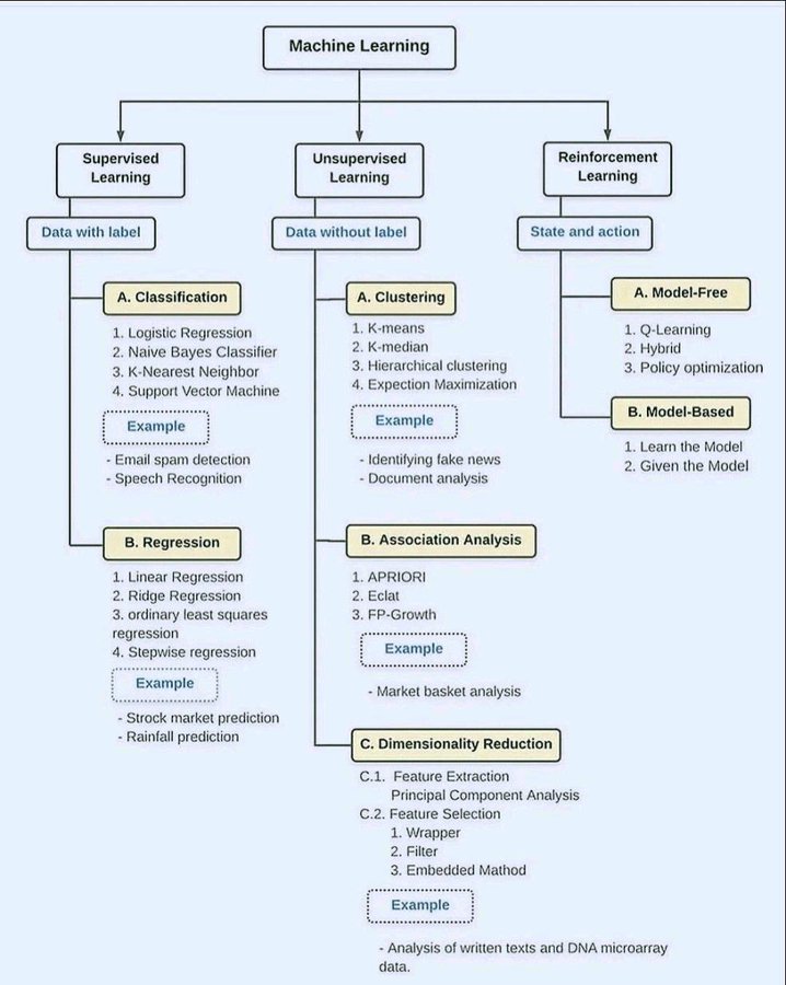
This article focuses on supervised machine learning. You’ll get an overview of the internals of the learning algorithm and features that you can use to train, score, and select the best-fitting prediction function.
Machine learning types and popular algorithms used

How machines learn to predict
The challenge of supervised machine learning is to find the proper prediction function for a specific question. Mathematically, the challenge is to find the input-output function that takes the input variables x and returns the prediction value y. This hypothesis function $h_{\theta}$ is the output of the training process. Often the hypothesis function is also called target function or prediction function or model.
$$y=h_{\theta}(x)$$
where;
- $h_{\theta}(x)$: hypothesis function, target function, prediction function, model
- $x$: feature parameter or vector
- $\theta$: theta parameter or vector
x represents a multiple-data point ${x_1, x_2, …}$ such as { 101.0, 3.0 }. The array of these values is referred to as the feature vector.
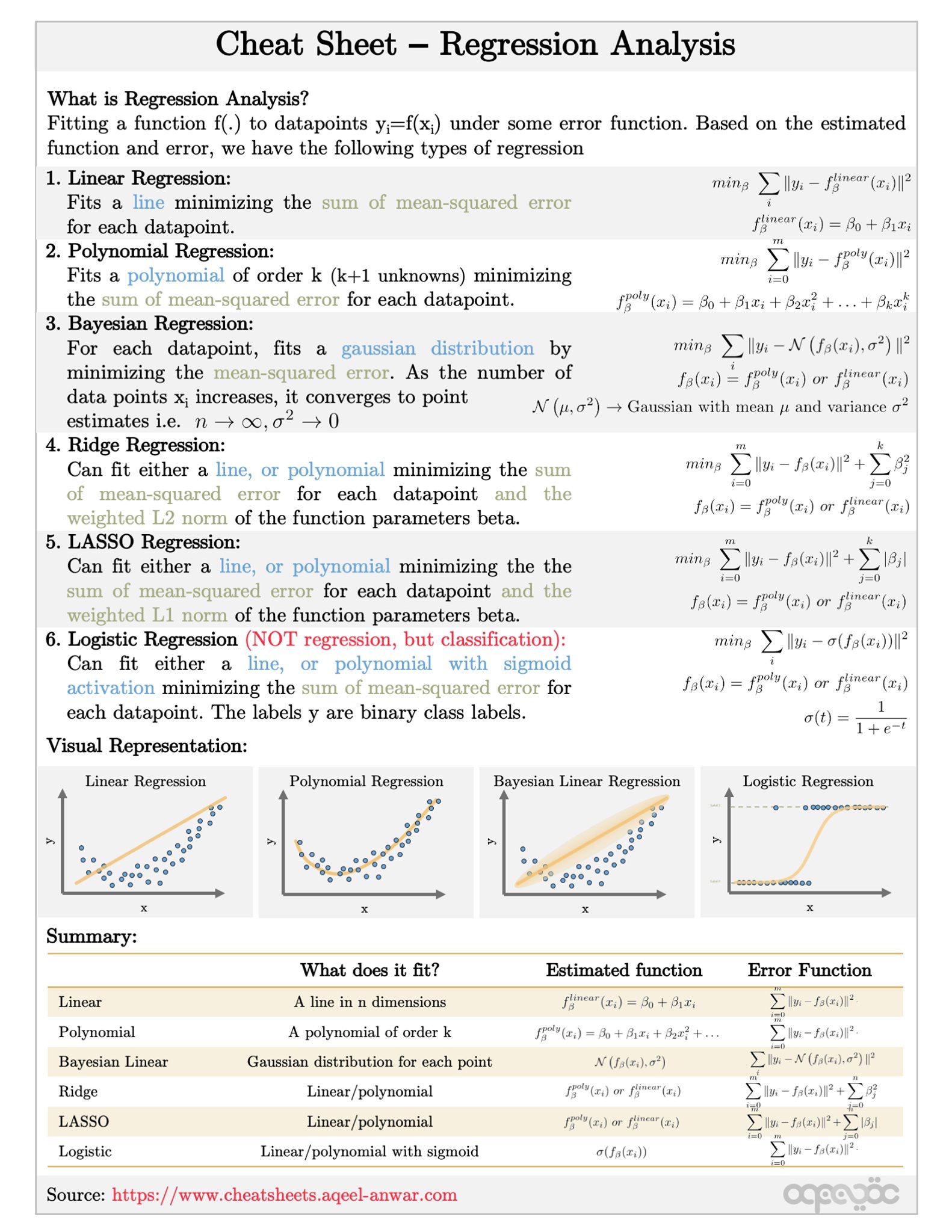
Linear regression

The generic linear regression function below returns the predicted value by summarizing each element of the feature vector multiplied by a theta parameter $(\theta)$. The theta parameters are used within the training process to adapt or “tune” the regression function based on the training data.
$$h_{\theta}(x) = \theta_{0} * x_{0} + \theta_{1} * x_{1} + … + \theta_{n} * x_{n}$$
In the linear regression function, theta parameters and feature parameters are enumerated by a subscription number. The subscription number indicates the position of theta parameters $(\theta)$ and feature parameters $(x)$ within the vector. Note that feature $x_0$ is a constant offset term set with the value $1$ for computational purposes.
How do you know that this theta vector is the best fit for your application? Would the function fit better if you changed the first or second theta parameter? To identify the best-fitting theta parameter vector, you need a utility function, which will evaluate how well the target function performs.
Scoring the target function
In machine learning, a cost function $J(\theta)$ is used to compute the mean error, or “cost” of a given target function.
$$J(\theta) = \frac{1}{2*m} * \sum_{i=1}^{m} (h_{\theta}(x^{(i)}) - y^{(i)})^2$$
The cost function indicates how well the model fits with the training data. To determine the cost of the trained target function, you would compute the squared error of each sample ($i$). The error is the distance between the calculated $y$ value and the real $y$ value of the sample $i$. The smaller the cost value of $J(\theta)$, the more precise the target function’s predictions will be.
Training the target function
Although the cost function helps to evaluate the quality of the target function and theta parameters, respectively, you still need to compute the best-fitting theta parameters. You can use the gradient descent algorithm for this calculation.
Gradient descent
Gradient descent minimizes the cost function, meaning that it’s used to find the theta combinations that produces the lowest cost ($J(\theta)$) based on the training data.
Here is a simplified algorithm to compute new, better fitting thetas:
$$ repeat { \ \theta_{0} := \theta_{0} - \alpha * \frac{1}{m} * \sum_{i=1}^{m} (h_{\theta}(x^{(i)}) - y^{(i)}) * x_{0}^{(i)}, \ \theta_{1} := \theta_{1} - \alpha * \frac{1}{m} * \sum_{i=1}^{m} (h_{\theta}(x^{(i)}) - y^{(i)}) * x_{1}^{(i)}, \ \theta_{n} := \theta_{n} - \alpha * \frac{1}{m} * \sum_{i=1}^{m} (h_{\theta}(x^{(i)}) - y^{(i)}) * x_{n}^{(i)} \ } $$
Within each iteration a new, better value will be computed for each individual $\theta$ parameter of the theta vector. The learning rate $\alpha$ controls the size of the computing step within each iteration. This computation will be repeated until you reach a theta values combination that fits well.
To validate that the cost decreases continuously, you can execute the cost function $J(\theta)$ after each training step. With each iteration, the cost must decrease. If it doesn’t, then the value of the learning rate parameter is too large, and the algorithm will shoot past the minimum value. In this case the gradient descent algorithm fails.
Although the cost will no longer decrease significantly, the target function is still not optimal; it seems to underfit. In machine learning, the term underfitting is used to indicate that the learning algorithm does not capture the underlying trend of the data.
From this we conclude that the model used for the training process, the target function, does not fit the data well enough. Underfitting is often due to an excessively simple model.
Adding features and feature scaling
If you discover that your target function doesn’t fit the problem you are trying to solve, you can adjust it. A common way to correct underfitting is to add more features into the feature vector. Rather than using the single domain-specific feature vector ({size} for example), you could use a multi-valued feature vector ({size, number-of-rooms, age} for example).
In some cases, there aren’t enough features in the available training data set. In this case, you can try adding polynomial features, which are computed by existing features.
$$h_{\theta}(x) = \theta_{0} * x_{0} + \theta_{1} * x_{1} + \theta_{2} * x_{2}^{2}$$
$$h_{\theta}(x) = \theta_{0} + \theta_{1} * \text{size} + \theta_{2} * \text{size}^{2}$$
Using multiple features requires feature scaling, which is used to standardize the range of different features. For instance, the value range of $\text{size}^{2}$ feature is a magnitude larger than the range of the size feature. Without feature scaling, the $\text{size}^{2}$ feature will dominate the cost function. The error value produced by the $\text{size}^{2}$ feature will be much higher than the error value produced by the size feature. A simple algorithm for feature scaling is Mean Normalization:
$$x^{’} = \frac{x-avg(x)}{max(x)-min(x)}$$
where $x^{’}$ is the normalized value. Mean normalization is used to rescale each sample.
As you add more and more features, you may find that the target function fits better and better. If you add too many features, you could end up with a target function that is overfitting.
Overfitting and cross-validation
Overfitting occurs when the target function or model fits the training data too well, by capturing noise or random fluctuations in the training data. Although an overfitting model matches very well on the training data, it will perform badly when asked to solve for unknown, unseen data. To avoid overfitting:
- Use a larger set of training data.
- Use an improved machine learning algorithm by considering regularization.
- Use fewer features.
If your predictive model overfits, you should remove any features that do not contribute to its accuracy. The challenge here is to find the features that contribute most meaningfully to your prediction output.
Overfitting can be identified by visualizing graphs. Even though this works well using two dimensional or three dimensional graphs, it will become difficult if you use more than two domain-specific features. This is why cross-validation is often used to detect overfitting.
In a cross-validation, you evaluate the trained models using an unseen validation data set after the learning process has completed. The available, labeled data set will be split into three parts:
- The training data set.
- The validation data set.
- The test data set.